


Next: 2.3 The confirmation algorithm
Up: 2. The filtering procedure
Previous: 2.1 First selection
2.2 The checking algorithm
In the second filtering stage we propagate the orbit to the exact time
of the attributable, rather than the rounded time used in the first
stage. As the time of the attributable we use the central time tm
defined above. The attributable contains the values of
 and
and
 as derived from the linear fit, but also the slopes
of the same fit, that is the proper motions
as derived from the linear fit, but also the slopes
of the same fit, that is the proper motions
 and
and
 ,
which provide the rate of motion on the plane
tangent to the sky. This information allows us to perform the
comparison with the predictions in a four dimensional space.
The orbit is propagated with the full variational equations, in such a
way that the covariance of the predictions can be computed (see
[Milani 1999], Section 3.1). Let
,
which provide the rate of motion on the plane
tangent to the sky. This information allows us to perform the
comparison with the predictions in a four dimensional space.
The orbit is propagated with the full variational equations, in such a
way that the covariance of the predictions can be computed (see
[Milani 1999], Section 3.1). Let
 be the
 covariance matrix of the predicted angles
 and
and
 the corresponding
normal matrix. Since it is better at this stage to use a prudent
estimate, we assume that the observation errors could be comparatively
large, e.g., with an RMS
the corresponding
normal matrix. Since it is better at this stage to use a prudent
estimate, we assume that the observation errors could be comparatively
large, e.g., with an RMS
 arc seconds. Then, the
covariance matrix expressing this assumed uncertainty in the
plane is
arc seconds. Then, the
covariance matrix expressing this assumed uncertainty in the
plane is
let
 be the corresponding normal matrix.
Then, the likelihood that the predicted and the attributable
observations are indeed the same can be expressed by the 2-dimensional
penalty [Milani et al. 2000a]
be the corresponding normal matrix.
Then, the likelihood that the predicted and the attributable
observations are indeed the same can be expressed by the 2-dimensional
penalty [Milani et al. 2000a]
Since the proper motion data are also available, let
 be the covariance matrix of the predicted
proper motions
be the covariance matrix of the predicted
proper motions
 ,
and
,
and
 the normal
matrix. The uncertainty of the proper motions as estimated from
observations depends upon the length
the normal
matrix. The uncertainty of the proper motions as estimated from
observations depends upon the length  of the observed arc:
 .
Then the covariance
matrix expressing this assumed uncertainty in the
plane is
.
Then the covariance
matrix expressing this assumed uncertainty in the
plane is
and, with
 ,
we can use the same 2-dimensional
penalty:
,
we can use the same 2-dimensional
penalty:
The two penalties have to be combined to assess the likelihood of the
attribution: we use
because each penalty is an increase in the value of the target
function, which is related to the square of the residuals (in this
case the residuals are the difference between the prediction for the
given orbit and the observation of the given attributable). It would
be possible to use a full 4-dimensional penalty, taking also into
account the correlation between predicted angles and proper motions,
but this does not appear to be necessary.
The computational cost of the second stage is much less than that of
the first one, essentially because the number of pairs
orbit-attributable to be tested has been decreased by three orders of
magnitude by the first filter. As an example, during the May 2000
update we have used about 7 CPU hours.
The geometrical meaning of this method is the following. The
observation as given in the attributable has an unknown error; the
real one could be anywhere within a distance of the order of
 ,
along great circles on the sphere (the factor
,
along great circles on the sphere (the factor
 correctly accounts for the metric on the sphere); this
is analytically described by the normal matrix Cobs. The
prediction is in turn uncertain, its confidence region being the
ellipse defined by the normal matrix
correctly accounts for the metric on the sphere); this
is analytically described by the normal matrix Cobs. The
prediction is in turn uncertain, its confidence region being the
ellipse defined by the normal matrix
 .
We are looking for
intersections of the two confidence regions. This situation is mathematically
the same as the identification problem in the elements space, only in
two dimensions. The same argument applies to proper motions.
.
We are looking for
intersections of the two confidence regions. This situation is mathematically
the same as the identification problem in the elements space, only in
two dimensions. The same argument applies to proper motions.
Figure:
Histogram of the number of attributions,
submitted by us and published by the MPC, as a function of the control
parameter  of the checking algorithm.
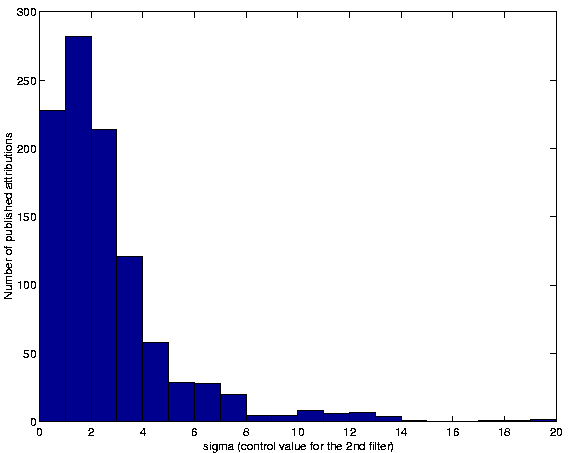 |
It is not easy to decide a priori the control value
to be
used for confirming the proposed attribution and passing it to the
final differential correction procedure. Figure 1 shows
the values of
for the attributions which have been accepted
by the MPC. Note that during the April update we have ourselves
selected for differential corrections all the cases with  ,
but only
,
but only
 of these have
 .
Among the pairs
later passing the third filter, only
.
Among the pairs
later passing the third filter, only  had
.
This means the control value can be kept very low, and we actually
plan to use a lower value in the future. The number of good cases
that could be missed by decreasing the control value would be small:
as shown in Figure 1, the number of published
attributions with
had
.
This means the control value can be kept very low, and we actually
plan to use a lower value in the future. The number of good cases
that could be missed by decreasing the control value would be small:
as shown in Figure 1, the number of published
attributions with  is just 5 (including one case out of
scale in the plot, with
is just 5 (including one case out of
scale in the plot, with
 ).
From Table 1 we can infer that the fact of passing
the second filtering stage with a low value of
has a good
predictive value for attributions to multi-opposition and
medium arc (
).
From Table 1 we can infer that the fact of passing
the second filtering stage with a low value of
has a good
predictive value for attributions to multi-opposition and
medium arc ( days) orbits; that is, a significant fraction
of the pairs passing the second filter are also passing the third
filter. However, for shorter arcs the second filter is not so
effective and a very significant computational effort has to be used
in the third stage; this can be understood as follows.
For short arc orbits, the confidence boundary of an observation
prediction, many years after the asteroid has been lost, is typically
several degrees long. Then the ratio between the area in which the
attributables are passed by the first filter (
days) orbits; that is, a significant fraction
of the pairs passing the second filter are also passing the third
filter. However, for shorter arcs the second filter is not so
effective and a very significant computational effort has to be used
in the third stage; this can be understood as follows.
For short arc orbits, the confidence boundary of an observation
prediction, many years after the asteroid has been lost, is typically
several degrees long. Then the ratio between the area in which the
attributables are passed by the first filter (
 square degrees) and the area A2 of the confidence
region acceptable for the second filter is roughly
square degrees) and the area A2 of the confidence
region acceptable for the second filter is roughly
where  is the width of the confidence region, which can be
computed as the square root of the lower eigenvalue of
is the width of the confidence region, which can be
computed as the square root of the lower eigenvalue of
 .
For R=1.5 degrees and a control value of the second filter
.
For R=1.5 degrees and a control value of the second filter 
This simple order of magnitude computation shows that for a width of
the confidence region of the order of several arcmin the second filter
becomes ineffective. If the available computing resources are not
enough, a decrease in the control value of
is an acceptable
compromise, in particular for short arc orbits: it would result in a
significant decrease of the computational load of the third stage,
with the possible loss of a small fraction of the real attributions
detected.
Next: 2.3 The confirmation algorithm
Up: 2. The filtering procedure
Previous: 2.1 First selection
Andrea Milani
2001-12-31