3.1 Nominal orbit and Modified Target Plane

The first step is to solve for the orbit of 1997 XF₁₁ by using only the observations between the discovery, in December 1997, and March 4, 1998; these were the observations available on March 11, 1998. Before applying the confidence boundary methods discussed in this paper we need to check the hypothesis, introduced at the beginning of Section 2, that the least squares fit results in a well determined solution, with a confidence region small enough to allow for the use of the confidence ellipsoid as a good approximation to the confidence region. After solving for the orbit with 98 observations, from 12 different observatories, the RMS of the residuals is 0.61arc seconds; after discarding 5 outliers in 2 iterations of removal at the 3 RMS level, the solution with 93 observations has an RMS of 0.50 arc seconds. The conditioning number of the covariance matrix is $232\,000$ (in non singular equinoctal elements), with a largest eigenvalue $\sigma_1^2=3.9\times 10^{-9}$, thus the confidence ellipsoid is quite small and is a good approximation.

  

Figure: Residuals (arc seconds) in right ascension (top) and in declination (bottom) for the orbital fit of 1997 XF₁₁ by using only the 1997-98 observations; on the horizontal axis, time in days from 1/1/1998. The discarded observations (because either $\alpha$ or $\delta$ has a residual larger than 3 times the RMS) are marked with circles. Continuous lines join the observations from the same professional observatory, dotted lines join the ones from the same amateur observatory.

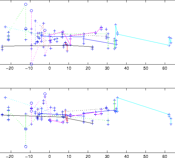The residuals after this second fit are plotted in Figure 2; the fact that the residuals from each individual observatory are not Gaussian is quite apparent. Nevertheless the errors of the different observatories do not appear to have a common bias/trend, as it reasonable since an asteroid observed near the Earth is not seen always in the same region of the sky, were regional star catalogue errors are expected to be systematic. Adopting the method described in Paper I, Section 2.2, and universally used in the astrodynamics/satellite geodesy applications, we select a weighting scheme such that the non discarded observations are very unlikely to have errors above 3 times the normalized scale (which is the inverse of the weight).

By inspection of the Figure 2, it is clear that a reasonably prudent choice is to use a scale of 1 arc second, that is equivalent to using a safety factor about 2 with respect to a naive application of the Gaussian statistics to non Gaussian errors. Thus all the normal and covariance matrices used in the following are computed with weight unity (in arc seconds), and incorporate this safety factor. We have to acknowledge that this choice of weighting is not an exact science; e.g. an argument could be proposed to use a safety factor $\sqrt{no.observations/no.observatories}=\sqrt{93/12}=2.78$; as we will see, the results of Figure 7 might be used to argue that a somewhat higher safety factor would give a better agreement. The possible values of the weighting scale are anyway not very different, and the discussion of the following results would not be significantly affected, apart from the discussion of Figure 7.

Then we compute the nominal orbit, solution of the least squares fit, until the year 2028, and find the closest approach position and velocity, which is at a distance of $0.000\,29$ AU from the center of the Earth on October 26, 2028; the planetocentric velocity is 14.6km/s, and the unit vector along this velocity is used to define the Modified Target Plane. By using the multiple solution formalism (described in Paper I, section 5) it is possible to find solutions compatible with the observations passing at about 3 Earth radii from the surface of the Earth. Note that, the close approach being very deep, some caution is needed to compute the orbit and to find the closest approach point with the required accuracy.

For numerical integration we have used the Runge-Kutta-Radau scheme [Everhart 1985], with adaptive stepsize change when stronger perturbations are encountered. This method performs well even in presence of close approaches, but for the deepest ones it sometimes fails to achieve convergence in the standard 2 iterations. We have modified the algorithm allowing for a variable number of iterations.

The dynamic model for a refined close approach analysis must be very accurate; all the results of this paper about 1997 XF₁₁ are based upon a model including the general relativistic perturbations from the Sun, the gravitational perturbations from the 3 largest asteroids, but not the gravitational perturbations due to the Moon. We have checked that the inclusion of the gravitational effects of the Moon would not change significantly the results: e.g. the nominal closest approach distance for the 1997-98 orbit would be $0.000\,27$AU, only $3\,000$ km less, due to the displacement of the center of the Earth from the center of mass of the Earth-Moon system.

The algorithm to determine the closest approach point is based upon an iterative regula falsi method to find the zero of the radial derivative (with respect to the approached body); the regula falsi is activated whenever a change in sign of the radial derivative is detected, and the following substeps are computed independently from the prosecution of the orbit integration, with a different algorithm, Runge-Kutta-Gauss [Butcher 1987], which is known to be especially stable in hyperbolic orbits. The MTP crossing is detected with the same method, applied to the derivative of the $\xi$ coordinate (see Section 2).